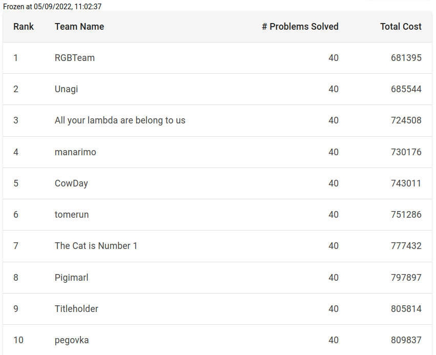
For the third year in a row, I participated in the ICFP Contest as a member of RGBTeam with Roman Udovichenko and Gennady Korotkevich. We won it last year and hopefully did a good job this year as well. The final results are not published yet, but we were in the first place when the scoreboard was frozen (2 hours before the end of the contest). Obviously, some teams could have submitted better solutions during the freeze, so the final results could be a little different.

One of the differences between the ICFP Contest and other competitions is that problem is prepared by different people every year, so you get a unique experience each time. This year’s task was quite straightforward (say, compared to two years ago), but still quite interesting and challenging. So thanks a lot to the organizers for preparing it!

Problem

The detailed problem statement could be found here, but let me briefly describe it. You were given a picture, which you need to draw by doing some operations. Initially, you start from one empty rectangle (actually, that was not true for some of the tasks, but more on that later), and can do some operations:

• Split a rectangle into two by a line, which is parallel to the X or Y axis.
• Split a rectangle into four by two lines parallel to the X and Y axis.
• Merge two adjacent rectangles. It is only allowed if the merged figure is still a rectangle.
• Fully color one rectangle.
• Swap two rectangles. It is only allowed if both rectangles have the same size.

When you merge or split rectangles, previous rectangles are destroyed and you can’t refer to them anymore.

Each type of operation has some cost associated with it. Also, the cost of the operation is divided by the area of the rectangle it is applied to (in the case of a merge operation — the area of the biggest rectangle). So coloring the whole canvas is very cheap (because we divide by the big area), and coloring one pixel is very-very expensive.

This cost function seems controversial, but probably the idea was to force participants to use big rectangles to create pictures, which are still similar to a very detailed picture.

After you have done all operations, the generated picture is compared to a target one pixel by pixel. The difference between two pixels is calculated as the Euclidian distance between RGB values:

\[0.005 \cdot \sqrt{(r_1 - r_2)^2 + (g_1 - g_2)^2 + (b_1 - b_2)^2}\]

To calculate the final score, you need to sum the cost of all operations and the differences between all pixels. A lower score is better. Here is an example of the target picture and picture produced by some operations with a total score of 17139.

In total there were 40 different tasks, and the overall score is just a sum of scores for each task.

Initial approach

This problem could be solved by dynamic programming. For each state (x_left, y_bottom, width, height) we can calculate the optimal scoring function. Transitions are simple:

• Fully color this rectangle.
• Split rectangle by line into two. In this case, you need to calculate the sum of scores for two smaller dp states and the cost of the split operation.

There are O(N^4) states in this dp, where N is the width/height of the picture (which was 400). When we fully color the rectangle, we need to calculate the sum of distances for all pixels in this rectangle, which can be done in O(N^2). So naively this algorithm requires O(N^4) memory and does O(N^6) operations, which are quite big numbers for N=400.

But we can optimize this algorithm by reducing the N. Instead of running it on the initial picture, we can first split the picture into blocks of size 10x10, for each block calculate the average color, and then run the algorithm on the picture of size 40x40. Of course, it will not find the optimal answer, and will only draw rectangles with coordinates, which are multiple of 10, but at least it could finish in a reasonable amount of time.

And if you are ready to wait, you can use blocks of smaller size instead of 10x10. You can also optimize performance a little bit by not calculating scores for some transitions/states. For example, if you have considered splitting the rectangle into two and know the best possible score, and now trying to check if just coloring the whole rectangle could lead to a better score. You can start iterating through all pixels in this rectangle and calculate the sum of distances with the target picture. But if the sum already exceeds the best score from splitting, you can stop there, and not consider this move. Or you can do some kind of estimations like “consider 10% of random pixels, approximate the score, only fully recalculate if it is good enough”. Such optimizations could speed things up a little bit, but not dramatically (you still can’t run dp on the whole 400x400 picture).

Scoring function

As I already mentioned the cost of operations is calculated by a little bit strange formula when you pay proportional to the inverse of the rectangle area. Let’s say we just want to draw a single pixel (x, y) in the middle of the canvas. The Naive way to do this looks like this:

1. Split the canvas by (x, y).
2. Split the top-right part by (x+1, y+1).
3. Pixel (x, y) is a separate rectangle now, so we can color it.

The third operation costs a lot as the area of the colored rectangle is just 1.

Instead, we can have a longer sequence of moves, but which doesn’t require operations with small rectangles:

1. Split by (x, y).
2. Fully color the top-right rectangle.
3. Split the top-right rectangle by (x+1).
4. Color the right part of it white.
5. Split the left part by (y+1).
6. Color the top part of it white.

There is a problem with the second approach. If something was already drawn in the top-right corner, it will be cleared by our operations. So we can’t use it naively to draw all rectangles. But we can always sort all rectangles we want to draw in a way that drawing each new rectangle doesn’t cause any problems to all the previous ones.

In this approach, we don’t even need to do operations 3-6. We can always assume there will be some later rectangle, which will recolor the top-right corner correctly.

To summarize, our algorithm will look like this:

• Split the whole picture into rectangles, where each rectangle will be colored into one color.
• Sort rectangles by some magic comparator.
• For each rectangle in order, color it and the area to the top-right of it into one color. This is done by splitting the whole canvas by the left-bottom corner of the rectangle, coloring one part, and merging all parts into one big rectangle back.

Local optimizations

ICFP Contest is usually 72 hours long, and the first 24 hours are usually called lightning division. There is a special “prize” for being the first on the leaderboard after the first 24 hours, so you want to have some working solution for this moment.

After the first ~20 hours, we had a solution similar to what is described above. It used some dynamic programming, and the trick to color rectangles. It gave us a pretty decent score, but still quite far from first place.

As I already wrote in a previous post (sorry, in Russian), local optimizations are a really powerful technique. It is quite common in marathon-style contests, that you generate some reasonable solution first, and then try to iteratively change it a little bit to improve the score.

To be able to do local optimizations, we need to represent our solution in a way that small changes to the solution don’t lead to a completely different resulting picture. For example, if we represent the solution as just a sequence of applied operations and try to add/delete some operations, it will not work very well as inserting one operation could completely change the meaning of the next operations.

Instead, we can represent our solution as just a list of bottom-left corners of rectangles with their colors. This list is sorted in an order in which rectangles are drawn.

We can start by picking a random corner from the list, and moving it by 1 in a random direction. If we get a solution with a better score, we leave a corner in a new place, otherwise, move it back. And trying to do this operation in a loop while the score improves.

This alone works pretty well. One of the reasons is explained by how we build our initial solution. We used a dp, which doesn’t have one-pixel precision, instead, all coordinates are rounded to the closest block size. So if the target picture contains some “border” between two objects, our dp probably guessed this border incorrectly by a couple of pixels.

We can also try to delete existing corners or add new ones in our local optimizations. But adding new corners doesn’t work well, because we need to guess a good position for a corner, and the probability of it is pretty low.

Color picking

Another optimization that we made before the 24-hour mark is picking a better color for each “color” operation. Initially in dynamic programming, when we want to fully color a rectangle, we just used an average of all target pixels lying in that rectangle. But this is not optimal.

Let’s consider a simple case of the rectangle consisting of one pixel with color (255, 0, 0) and 10 pixels with color (0, 0, 0). For such a case, we can only consider the first coordinate (red) as others are equal to zero. The weighted average of the red component is (255 + 0 * 10) / 11 = 23. And the cost of this rectangle is 10 * 23 + 1 * (255 - 23) = 462.

Instead, we can just use color (0, 0, 0) for this rectangle. And the score for this color will be 10 * 0 + 1 * 255 = 255. Which is much better than 462!

Finding the best color in the general case is actually a known problem called Geometric median. Wiki suggests there is a Weiszfeld’s algorithm, which can be used for solving it. In the end, some of our solutions used it, but we started with a simpler algorithm, which is Local optimizations (again).

Let’s start with a weighted average color (which is a good approximation to a correct answer), and then try to change one of the (red, green, blue) components by one in one of two directions. After changing, we recalculate the cost, and, if it is better than before, continue with a new color. If we tried all 6 possible changes and none of them led to a better answer, we stop.

This algorithm is very easy to code, but actually works pretty fast and, I believe, always finds the best color.

Local optimization improvements

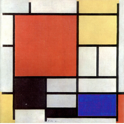
To show how good local optimizations work, let’s just look at one example. Here is a target picture for test 21:

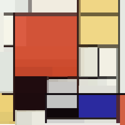
Here is a solution generated by dynamic programming with block_size = 6. Score = 22087.

And here is the same solution after local optimizations. The score is 14653.

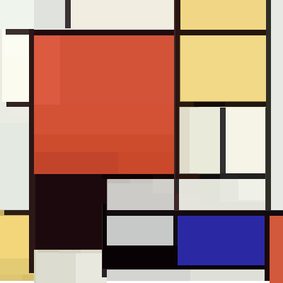
Maybe the difference in the generated pictures is not that big, but the difference in scores is really huge! The best answer found for this test during the whole competition is 12567, which is not that far from 14657 found by 10 seconds of local optimizations.

The results of the lightning division are currently not published yet, but I am pretty confident that we won it by a huge margin (thanks again to local optimizations!).

Merging

After the lightning division finished, there was a small modification to the problem statement, and new tests were added. The difference was that in new tests the initial canvas is not empty. Instead, it was split into squares of different colors.

I am not sure what was the expected way of handling new cases, but when we saw this modification, we almost instantly decided that we just need to merge all squares into the big one, clear it, and draw the picture as we did in previous tests.

Merging all squares into one seemed like not a very hard task. We can just merge each line separately, and then merge lines together. So we coded this pretty fast and got some scores.

We also wrote a tool to show the top scores for each test. It looked like this:

I should also mention that all new tests had target pictures that exactly matched the target pictures of previously known tests. For example, the target picture for test 32, which is shown above, is absolutely the same as for test 9. At some point, we saw a team CowDay, which had a score on new tasks, which is much lower than we spent on just merging all squares together (not including an additional cost we pay to actually draw a picture after merging). There were two possible options:

• They do not merge squares, and instead, use them to draw a target picture somehow.
• They learned how to pay less for merging.

We checked the difference between their scores for new tests and corresponding old tests. And for both tests where the initial canvas is split into 20x20 squares, the difference was 19877, which could not be a coincidence. So probably they merged squares more efficiently (we spent 28451 on merging), but how?

After quite some time of thinking, we realized that when merging squares together, it is sometimes important to use the “cut” operation!

As I already mentioned, the cost of operations is proportional to the inverse of the rectangle area. So we want to reduce the number of operations with small rectangles. When we naively merge each line separately, we start each line by merging two small squares, which costs a lot. Instead, we can do something like:

• Merge the first 7 rows separately.
• Merge them into one big 7x20 block.
• Split this 7x20 block into 20 blocks of size 7x1.
• For each 7x1 block add 13 more cells, so now we have 20 columns of size 20x1.
• Merge all 20 columns together.

This is how it works for a 16x16 case.

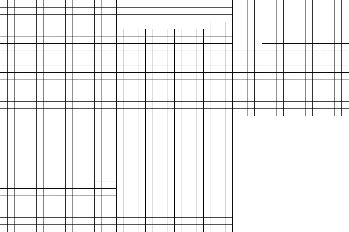
This way requires more operations than the naive one, but it only uses 7 very costly operations instead of 20. The cost of this way is 19872, which almost matched the difference the CowDay team had in their scores, so looked like we found the same way as them.

After some time we noticed that team Unagi does something even more clever with the cost of 17571.

In the end, we realized we can generalize our solution to use several steps:

• Build first A rows.
• Build first B columns.
• Build next C rows.
• Build next D columns.
• …

Values (A, B, C, D, ...) could be computed with dynamic programming. The state of the dynamic programming is (we built X first rows, and Y first columns, which are represented by two rectangles). There are two ways of representing a state as a union of two rectangles, so we also need to add an additional bit, which indicates it, to the state. And transitions are just adding some amount of new rows or columns.

Our final method for 16x16 looked like this:

Generating this sequence of operations looks like a nightmare, and I am very happy to have teammates who did this instead of me!

More optimizations

We also tried a number of other optimizations. Some of them improved the score, but not very dramatically.

• We used Simulated annealing instead of local optimizations in the end.
• We tried 4 possible rotations of the picture. In our solution, the top-right corner of the picture is very special, and drawing rectangles there cost a lot. So if we rotate a picture such that the top-right corner doesn’t contain complicated objects, it costs less.
• We tried to use the swap operation to move complicated parts of the picture far from the top-right corner. We did this mostly manually and improved the scores on a couple of tests. But based on other teams’ writeups, we underestimated the importance of this operation, and it could be used much more efficiently.
• We had a really nice visualization tool, which also supported some manual modifications of the solutions.

Infrastructure

It is not uncommon in ICFP Contest to use a lot of external computational resources as in most of the algorithms like simulated annealing if you give them more time, they will find a better solution.

But we decided to just use our 3 laptops to run our code. I think it forces you to write smarter algorithms, not rely on big servers :)

In terms of programming languages, I used Rust and my teammates used C++. We also had some tools written in Python.

Final thoughts

I enjoyed this year’s contest. There were a couple of technical issues during the contest, but they all were resolved. The problem was a little bit straightforward (e.g. our solutions didn’t change much since 24h mark), but still pretty interesting. Thanks a lot to the organizers!

Looking forward to the ICFPC 2023!