What is Simulated Annealing?

Simulated Annealing (SA) is the main algorithm in optimization-style programming competitions. Almost every Topcoder Marathon or Atcoder Heuristic Contest winner probably used SA. There are a lot of articles on the Internet about SA, so I’ll assume you already know the basics. I recommend this one.

The problem with all of them is that they explain the algorithm, but don’t share ideas about how to choose parameters. We will try to fix it in this blog.

Disclaimer: I myself don’t have a lot of experience with optimization style contests, so all facts in this blog should be taken with a grain of salt. But still, I was a member of the team, which won Google HashCode twice, where SA could be used in solutions.

Travelling salesman problem

In this blog, we will analyze the usage of SA for one specific instance of Travelling salesman problem (TSP). In TSP you are given n cities and distances between all of them. You need to find the shortest cycle, which visits every city exactly once. I took a specific TSP task from this old CodeForces post, it has 100 cities.

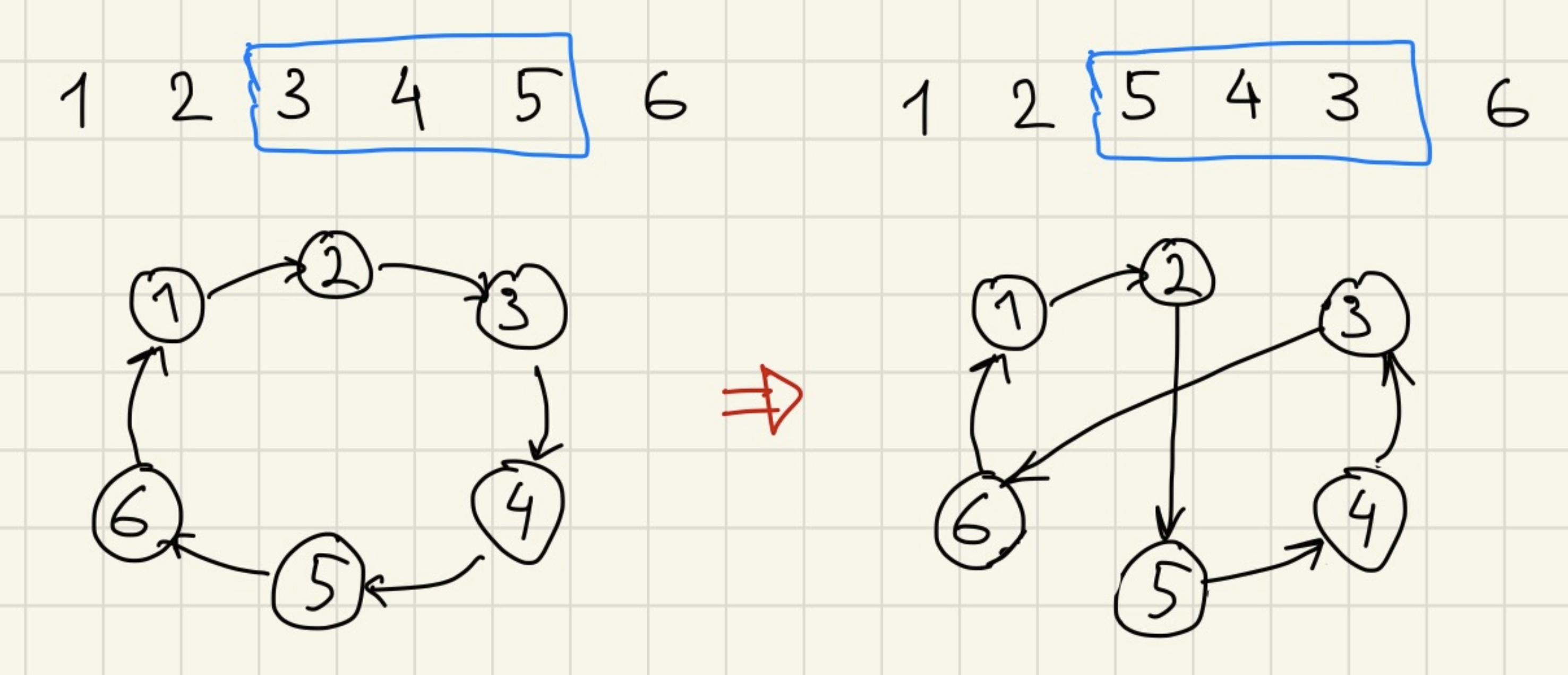
How can we use SA for solving TSP? First, we can say that the solution can be represented as a permutation of numbers from 1 to n – an order in which we visit cities. Second, we need to define possible transitions. In this case we will use a single possible change of the solution, which is called 2-opt. The idea is to take a random subsegment of our permutation and reverse it.

The code

Let’s write some code. The problem is in all posts about SA you can find different formulas, different temperature schedules, different <X>… What should we use?

Btw, I think this is exactly what stopped me from using SA in the past. There were so many tutorials, I picked a random one, it didn’t work well, and I just used different algorithms, which I knew, instead.

But now I know the right way. We can just take a look at how Psyho implements it :) I opened his code from the last Atcoder Heuristic Contest, and guess what I saw? Right, implementation of the SA.

So I wrote the code to solve TSP, which uses the same formulas (but with different temp_start and temp_end):

const MAX_SEC: f64 = 1.0;
let temp_start = 10.0f64;
let temp_end = 0.001f64;
let start = Instant::now();
let mut perm: Vec<_> = (0..n).collect();
let mut prev_score = calc_score(&dists, &perm);
loop {
   let elapsed_s = start.elapsed().as_secs_f64();
   if elapsed_s > MAX_SEC {
       break;
   }
   let elapsed_frac = elapsed_s / MAX_SEC;
   let temp = temp_start * (temp_end / temp_start).powf(elapsed_frac);
   let (fr, to) = pick_random_interval_to_reverse(n);
   perm[fr..to].reverse();
   let new_score = calc_score(&dists, &perm);
   if new_score < prev_score || fastrand::f64() < ((prev_score - new_score) / temp).exp() {
       // Using a new state!
       prev_score = new_score;
   } else {
       // Rollback
       perm[fr..to].reverse();
   }
}
let score = calc_score(&dists, &perm);
eprintln!("Score: {score}");

It is quite short! And it probably works better than most of the smart algorithms you can come up with!

There is some magic happens in the temp_start * (temp_end / temp_start).powf(elapsed_frac) and fastrand::f64() < ((prev_score - new_score) / temp).exp() parts. I’ll leave it as an exercise to you to understand them, but in fact you don’t need to know how they work. You can just copy it every time you want to use SA.

The really interesting part is just two simple lines:

let temp_start = 10.0f64;
let temp_end = 0.001f64;

How should we choose constants here? This time I just picked them kinda randomly from my experience, but this is not the advice you want, right?

Back to our TSP instance. We can run our code and get the result:

Score: 7.867000846582566

Is it good? Is everything ok? Can we do better? Should we change our constants?

It is hard to answer just from one number. We are not in a rush now, so we can visualize some data to get more insight into what could be improved.

Let’s visualize!

Disclaimer: there are a lot of plots in this post, and they are interactive (you can zoom into interesting parts). It is easier to interact with them on a device with a big screen. But if you still want to read it from the phone, consider rotating it to landscape mode and refreshing the page.

First, we can just draw a plot of the score depending on time.

It looks roughly as expected. We start from a random solution with a big score (total distance) and spend some time with a high temperature, which accepts bad transitions, so the overall score is still high. But as time goes on, temperature decreases and we slowly converge to a small score.

Sometimes it is also useful to draw several runs on the same plot to make sure all of them look similar.

Let’s take a closer look at what happens in the last 0.2 seconds.

Some thoughts:

For each specific run, the score at 0.8s is roughly the same as at 1.0s, which means we waste 20% of our time.
Different runs end at different scores (and different permutations), so running the algorithm several times could help find a better solution.

Save the best

Let’s optimize a single run. We can draw not only the current score, but the best score has seen so far:

For each point on the orange line, there should be a point from the blue line with the same score, which happened before. But we don’t see this happening on the plot, because points were sampled, and a lot of interesting blue points just were not lucky enough to stay on the plot.

And let’s zoom into what happens in the end:

The point, I want to illustrate here, is that if we terminate an algorithm at the wrong moment, and we use the last score instead of the best one (this is exactly what we do in the code above), we can get a much worse result, so always save the best result instead of the last.

Choosing parameters

Why do we spend the last 20% of the time doing nothing? Why do we spend the first 50% of our time with a very bad score?

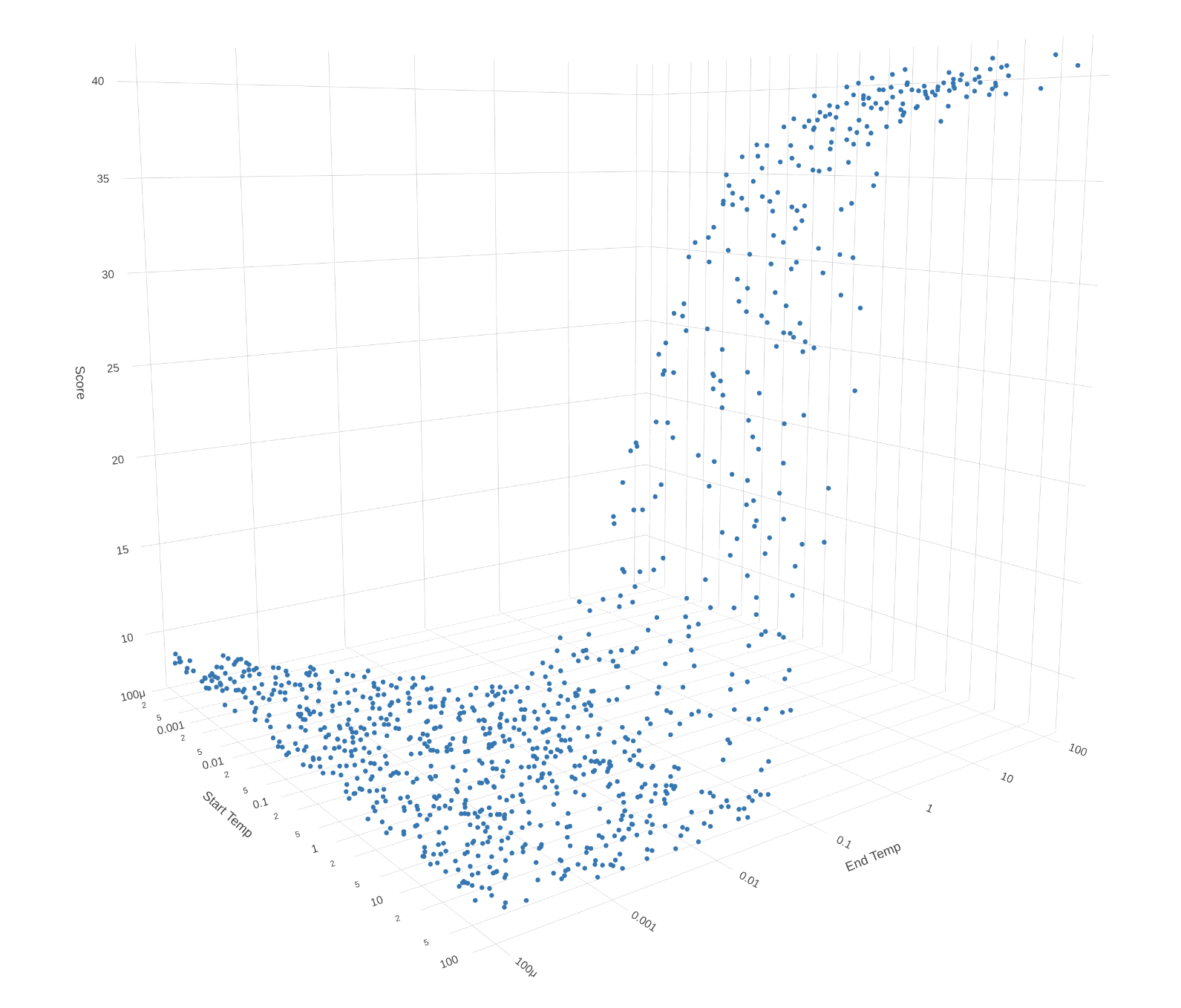
Let’s try to choose different temp_start and temp_end and see what score we get. We use logarithmic scales for the axis. And don’t forget that plots are interactive, so you can rotate them! Here each point represents one experiment.

Smaller scores are better, so the only conclusion we can definitely make is that temp_end should be smaller than 0.01 (otherwise we just accept bad transitions till the end and never get a good solution). Ok, let’s leave only smaller parameters, and rerun the experiment.

Ok, now let’s also say that temp_start should be at least 0.1 (otherwise we don’t explore the full space of solutions and just converge to some local optimum).

Now we see that after removing completely bad temperature parameters, results for all others look pretty random. We can also say that our initial randomly picked parameters temp_start = 10.0 and temp_end = 0.001 are inside the range.

Optimal answer

For this specific case of TSP, there is a known optimal answer, which we actually found several times. Let’s take a look at which start parameters this happens more often. I created a 10x10 grid with different temp_start and temp_end, for each cell ran 5000 experiments, and calculated the probability of finding the optimal solution.

From the previous plot, it was hard to compare “reasonable” start parameters, but now we can see some patterns.

For example, with big temp_start = 70 you still have chances to find the optimal answer, but this chance could be several times smaller compared to the optimal starting parameters. This probably happens because with high temp_start, we spend a lot of time accepting random changes instead of actually trying to find a good solution.

Now I think I have started to understand Psyho’s reply about choosing parameters. The starting temperature should be high enough to be able to visit all possible states, but not higher, because otherwise we just spend a lot of time picking a random starting point.

Let’s build the same Score(Time) plot as at the beginning for more optimal initial parameters (temp_start=0.2; temp_end=5e-3). And again we run the program several times to make sure all of the runs look similar.

The plot is quite different, right? Now we don’t spend the first half of the time on nothing.

10x1s or 1x10s?

From the previous heatmap, you can see that with optimal initial parameters, you can achieve the best score in ~3% of runs. This means on average you need to run your program 33 times (and spend 33 seconds) to get the optimal score. But maybe it is more optimal to run the program once, but for a longer period of time. Let’s check.

One thing to keep in mind is that we picked the best initial parameters for the 1s algorithm. Potentially, if we want to run it longer, the parameters should be different. But let’s not think about it for a while.

Single run time	Probability of finding optimal solution	Expected time to find optimal solution
0.1s	0.6%	16.5s
0.2s	1.3%	15.8s
0.5s	2.3%	22.1s
1s	3.0%	33.0s
2s	3.5%	57.5s
5s	6.4%	78.1s
10s	6.5%	153.8s

Well, in this specific problem, we can see that running an algorithm with a bigger Time Limit increases the probability of finding an optimal solution, but the overall effectiveness decreases. So it is even better to limit our algorithm to 0.2s, and run it more times than using our original 1s limit.

Intuitively it happens because the solution space is relatively small, and 0.2s is already enough for an algorithm to pick a good solution. But it is not always the case, for some bigger cases of TSP or for different problems, it is possible that running the algorithm once for a longer period is more optimal. So you always need to check what works better for a specific task.

Choosing parameters. Part 2.

We looked at how different starting parameters could affect the probability of finding the optimal solution. For example, there are some very bad choices (too small temp_start or too big temp_end), which lead to very bad results. But in other cases, results will probably be reasonably good.

For example, if you set temp_start to a very big value and temp_end to a very small one, then your algorithm will spend the first 40% of the time randomly changing the solution, and the last 40% doing no changes at all. But it will still spend the middle 20% the same way it would spend with optimal parameters. So if you can increase the Time Limit by 5 times, you will get the same result.

So if you are solving some specific task locally with SA, you can initially run it with very inefficient parameters, estimate what the score should be, and then try to move temp_start and temp_end closer to each other, and check that the score is still good enough.

We can use the fact that the function of the expected score depending on temp_start and temp_end is roughly independent by parameters, so you can first find an optimal temp_end, and then separately find an optimal temp_start.

Choosing parameters. Part 3.

But what can we do if we do not know the test case in advance? Or if the results are very noisy and it is hard to choose parameters.

Let’s look at another statistic. Whenever we consider applying some change, we can classify it into one of three categories:

It improves the score, and we apply it.
It makes the score worse, but we still apply it.
It makes the score worse, and we discard it.

We can track the moving average of the part of changes falling into categories (1) and (2).

This is how the plot looks like for our optimal temperature parameters (temp_start=0.2; temp_end=5e-3):

And this is for parameters we used at first (temp_start=10; temp_end=1e-3):

They look pretty different, right? And for different instances of TSP or even for different tasks, optimal plots will probably look similar to optimal plots for this task. So when choosing parameters for SA, we can build such a plot and try to make it look similar to the first one here.

I also think it should be possible to change the temperature automatically based on the acceptance rate, but I’ve never seen somebody doing this. Let me know if you tried it!

Performance optimizations

Usually, during optimization-style contests it is better to spend time trying different ideas, adding new types of transitions, and so on. Before doing any performance optimizations, try to just increase the time limit and check if it gives you a much better score.

But if you really decided to optimize performance, here are a couple of suggestions.

First, always print the number of checked transitions per second. Try to estimate how big this value should be, and compare it to the actual value, if it doesn’t match – investigate.

For example, let’s try to estimate what it should be for our TSP case. Every time we pick a random interval (which is O(1)), rotate this interval and calculate the score. Rotating and calculating the score is O(n), where n=100. So probably the total number of tries should be bigger than one million and smaller than ten million per second.

I actually wrote this guess before implementing the counter, so let’s see if I guessed correctly.

Average transitions checked: 10'040'966/s

So it is actually even faster than expected! But we can still check transitions in O(1). When reversing a subsegment of permutation, we only change two edges to two other edges.

This change is a little bit tricky and requires some carefulness, but it roughly looks like this:

let (fr, to) = pick_random_interval_to_reverse(n);
if to - fr + 1 >= n {
   // this change does nothing.
   continue;
}


let v1 = if fr == 0 { perm[n - 1] } else { perm[fr - 1] };
let v2 = perm[fr];
let v3 = perm[to - 1];
let v4 = if to == n { perm[0] } else { perm[to] };
// we replace edges (v1, v2) and (v3, v4) with (v1, v3) and (v2, v4)
let score_delta = dists[v1][v3] + dists[v2][v4] - dists[v1][v2] - dists[v3][v4];


let new_score = prev_score + score_delta;

After running it we can see:

Average transitions checked: 20'397'125/s

Well, it is two times faster, but it doesn’t look like O(n) vs O(1). We can run our program under perf and see this:

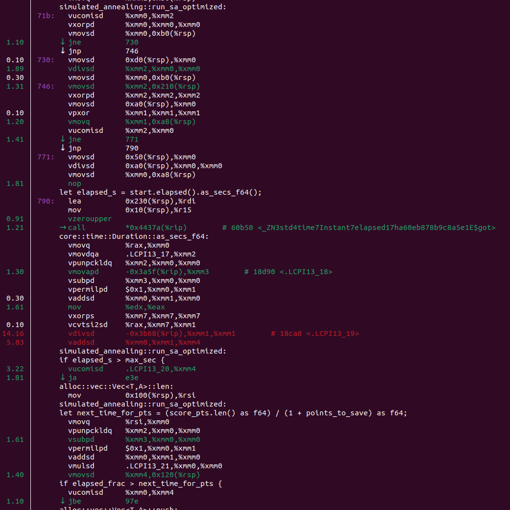
If you don’t understand asm, you still can see a suspicious core::time::Duration::as_secs_f64 there. And it is quite a common problem for SA. If your scoring function is O(1) and very fast, time measurement becomes the bottleneck. We need to measure time to calculate the current temperature and to determine when to stop.

The optimization is pretty simple. We can check elapsed time every 128 iterations, and just reuse the same value for the next iterations.

Now the loop looks like this:

let mut elapsed_s = 0.0;
for iter in 0.. {
   if iter & 127 == 0 {
       elapsed_s = start.elapsed().as_secs_f64();
   }
   ...
}

And now the performance is better:

Average transitions checked: 42'284'052/s

We can also cache the temp, because it requires a costly powf function:

Average transitions checked: 75'977'403/s

fastrand crate is pretty good, but we can still replace it with our own implementation of a simple xorshift random number generator:

Average transitions checked: 81'184'596/s

In our specific case, we can use hacky optimization. Let’s create a const N: usize = 100 (because we know the size of the input at compile time), and use it during random segment generation. To generate a number from 0 to n, we generate a 64-bit number and take it modulo n. If n is known during compile time, the compiler can replace the modulo operation with a faster instruction.

Average transitions checked: 90'212'640/s

Great! It is 9 times faster than the initial version. I also ran this version a lot of times with TimeLimit=0.02s and found that the probability of finding the optimal solution is 1.1% (which is similar to the not optimized version with TimeLimit=0.2s), and the expected time to find the optimal solution is now 1.8s, which is much better compared to the initial solution.

The end

Simulated Annealing is a big topic, and I definitely didn’t cover everything. The results could be very different if you will need to solve a bigger instance of TSP or a different task. But I hope you got some insights about how it works, and how to tweak parameters.

If you don’t want to read the full article, here is a short list of advice:

Always save the best-seen answer, not the last one.
Print the number of checked transitions and compare them to your estimations.
Draw/print stats about how often you accept bad transitions.
To pick temp_start and temp_end use very big and very small values to estimate the expected score. Then move them closer to each other until everything breaks dramatically.
Do not do premature optimizations. Before doing them, increase the TimeLimit and check if the score improves.
If you really want to optimize, make a score calculation O(1), cache the time and temperature, and optimize the random number generator.

You can check the source code of all the experiments on GitHub.

If you read till this point and know Russian, consider subscribing to my Telegram channel with similar posts: https://t.me/bminaiev_blog.

Borys Minaiev's blog

Contact

Converging on Simulated Annealing